Looking for new problems to solve? Consider the climate

Climate is not weather. As science fiction writer Robert Heinlein quipped, the chaotic and unpredictable nature of weather confounds our expectations, leading weather reporters on television to say regretfully “we should only get four inches of rain in September” as if the six inches that actually fell is a travesty of some sort. In reality, the weather is so sensitive to initial conditions that it isn’t possible to accurately predict it more than a week or two into the future. In contrast, the climate—the average weather—is describable and potentially predictable precisely because time averages wash out the details of the moment-to-moment weather. (This averaging effect has an analogy in the equation of state of an ideal gas, $PV=nRT$, which is indifferent to the individual motions of the molecules.)

Much effort in modeling the climate is focused on simulating the general circulation of the atmosphere and oceans. Climate models “spin up” from an initial state by integrating the equations of motion that describe the atmosphere or oceans forward in time, minute by minute, until they reach a statistical steady state. Statistics can then be accumulated by further integration. The method has yielded significant understanding, but as Edward Lorenz [2] at MIT observed more than 40 years ago:

“More than any other theoretical procedure, numerical integration is also subject to the criticism that it yields little insight into the problem. The computed numbers are not only processed like data but they look like data, and a study of them may be no more enlightening than a study of real meteorological observations. An alternative procedure which does not suffer this disadvantage consists of deriving a new system of equations whose unknowns are the statistics themselves.”

Lorenz was suggesting a direct statistical approach to the problem of climate that would refocus attention on the slowly changing degrees of freedom that are of most interest. These could include the mean temperature in a particular region, the position of storm tracks, or the typical size of fluctuations in rainfall. There is a catch, however: The approach requires the tools of nonequilibrium statistical mechanics, a discipline that remains poorly developed in comparison to its incredibly successful equilibrium cousin.

In this article, I discuss specific advances in nonequilibrium statistical physics that have direct applications on efforts to understand and predict the climate. (For an excellent introduction to the general science of climate change, see David Archer’s Global Warming: Understanding the Forecast [3].) But first, let’s look at the sort of question a statistical description of the climate system would be expected to answer.

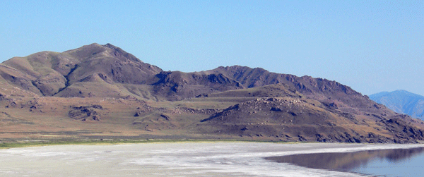
Reconstructions of past climate strongly suggest that the mean latitude of the global storm tracks shifted and/or changed in intensity about 10,000 years ago, as the last ice age came to an end. The shorelines of ancient pluvial lakes (that is, landlocked lakes that are filled by rainfall and emptied by evaporation) provide clues to where the storm tracks were once centered. The Great Salt Lake of Utah, for example, is in fact a remnant of a larger body of water called Lake Bonneville that covered the present-day salt flats during the last ice age (Fig. 1). Many of the ancient pluvial lakes throughout the American west, such as Lake Manly that once filled Death Valley in California, were the result of reduced evaporation combined with a southward shift of rain-bearing storms from their present day tracks.

Credit: Courtesy Mark Wilson/The College of Wooster

Credit: Courtesy Mark Wilson/The College of Wooster

×

The mean latitude and strength of the storm track are statistical quantities with important ramifications for future patterns of precipitation. In a warming climate, will the storms continue to migrate towards the poles, leading to drought at mid-latitudes? Will the storms strengthen or weaken? Short of waiting for the answer, the only way to proceed is by modeling the general circulation of the atmosphere. The models that do this run on supercomputers and can reproduce and predict shifts in the storm tracks, but (as Lorenz anticipated) it can be difficult to tease out the essential causes behind the shift. (For an insightful overview, see Isaac Held’s article, The gap between simulation and understanding in climate modeling [4]). The problem is very familiar to physicists that work on complex systems. The generally accepted procedure for modeling such systems is to begin with highly simplified models and add to their complexity only as the requirements of the physics dictate.

In this spirit, as a first approximation to modeling the complicated dynamics of the atmosphere and oceans, both fluids can be treated as quasi-two-dimensional. This simplification is based on observation: geophysical fluids are often highly stratified, moving for the most part in horizontal directions. Furthermore, these fluids are effectively incompressible. Such two-dimensional fluids have the nice feature that their motions are fully described by a single scalar vorticity field, the component of the curl of the velocity field pointing in the vertical direction,

and it is the behavior of such flows close to equilibrium that we turn to next.

Ocean currents show persistent large-scale flows that are especially vigorous along the eastern edges of the continents, such as the Gulf Stream and the Kuroshio current. These currents also spawn smaller rings or eddies that tend to propagate westward. The persistence of the flows suggests that even though they are driven by winds, they may be sufficiently close to equilibrium that equilibrium statistical mechanics could be a useful tool to understand their behavior.

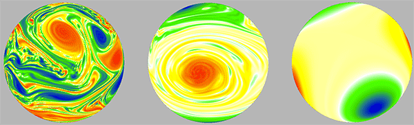
One striking feature of two-dimensional turbulent flows in such close-to-equilibrium conditions is that they organize spontaneously into large-scale and long-lived coherent structures, such as those seen in the far right panel of Fig. 2. In this direct numerical simulation, the equations of motion for the fluid on a sphere have been integrated forward in time, starting from a random distribution of vortices in the liquid that are equally likely to swirl in the clockwise (“negative”) and counterclockwise (“positive”) sense. Smaller vortices are swept along (“advected”) by the velocity fields of the larger ones and absorbed into them, until eventually only a quadrupole in the vorticity field remains [5]. In the limit of low viscosity, the change of the vortex field in time is governed by the equation of motion

subject to the incompressibility constraint $\nabla \cdot \mathbf{\text{v}}=0$. This is a nonlinear equation because the velocity field $\mathbf{\text{v}}$ is itself linearly dependent on the vorticity through Eq. (1). The term ${\nu }_2$ is called the “hyperviscosity.” Differently from the usual physical viscosity term ( $\nu {\nabla }^2\omega$) that normally appears in Eq. (2) to account for dissipation, the hyperviscosity is an artificial term that facilitates the numerical simulation. Namely, it addresses the fundamental limitation of all numerical simulations of low viscosity fluids: Driven by the nonlinearity, fluctuations in the vorticity cascade down to smaller and smaller length scales, eventually dropping below the resolution of any numerical grid. Hyperviscosity is a crude statistical tool for modeling this missing subgrid scale physics: it absorbs fluctuations at the small length scales, but hardly disturbs the total kinetic energy of the flow.

Credit: Wanming Qi and J. B. Marston (unpublished)

Credit: Wanming Qi and J. B. Marston (unpublished)

×

For flow patterns that develop in this way, the coherent structures that condense over time are largely independent of the details of the initial conditions. This suggests a simple interpretation in terms of equilibrium statistical mechanics. One such interpretation is based upon the variational principle of minimum enstrophy, as developed by Francis Bretherton and Dale Haidvogel [6] and by Cecil Leith [7]. Enstrophy is the mean square vorticity and it (along with an infinite number of higher moments) is conserved in the absence of forcing or dissipation. Viscosity, however, drives the enstrophy towards zero faster than the kinetic energy and this separation of time scales means that a nearly equilibrium state can be realized for some time before the energy slowly dissipates. This phenomenological approach captures in an intuitive fashion the physics of the inverse cascade process [8,9], whereby small-scale fluctuations organize into large-scale coherent structures, such as those seen in Fig. 2 and in Video 1.

More rigorous statistical mechanical formulations have also been constructed to describe fluids in the limit of zero viscosity. In such inviscid flows, finer and finer structures in the scalar vorticity field $\omega (\mathbf{\text{r}})$ develop as the fluid evolves. Jonathan Miller and his collaborators [10,11] and Raoul Robert and Joel Sommeria [12] (MRS) described the small-scale fluctuations of the fluid statistically, using a local probability distribution $\rho (\mathbf{\text{r}},\sigma )$ of vorticity $\sigma$ at position $\mathbf{\text{r}}$. The equilibrium state is then obtained by maximizing the Boltzmann entropy while conserving energy and the infinite number of other conserved quantities, namely the moments of the vorticity distribution. In the physical limit of small but nonzero dissipation, MRS argued that the vorticity field is adequately captured by the coarse-grained mean field

of the corresponding zero-viscosity theory, with dissipation acting to filter out the small-scale fluctuations.

However, treating dissipation in this way may not work well, because during the relaxation to equilibrium, viscosity can significantly alter the integrals of motion, especially the high-order moments. Recently, Aurore Naso, Pierre-Henry Chavanis, and Berengere Dubrulle [13] showed that maximizing the MRS entropy, holding only the energy, circulation, and enstrophy fixed, is equivalent to minimizing the coarse-grained enstrophy (the mean square of $\overline{\omega }$), as in the earlier minimum enstrophy theory. The result uses the statistical MRS theory to nicely justify the intuitive minimum enstrophy variational principle.

Peter Weichman in the US [14,15] and Freddy Bouchet and his collaborators in France [16–18] have applied these ideas to models of geophysical flows. The latter group has shown that transitions can occur between localized rings of vorticity and extended jets, mimicking behavior seen both in laboratory experiments and in ocean currents. Statistical mechanics descriptions of near-equilibrium flows have a distinct advantage over traditional numerical simulations, as transitions that occur on very long time scales that are inaccessible to direct simulation can now be studied. Whether or not actual oceanic flows are close enough to equilibrium for these approaches to apply remains an open question, however.

Of central importance to Earth’s climate is the difference in mean surface temperature between the tropics and the poles. The difference is determined by the differential heating of the Earth’s surface (more solar radiation falls at the equator than near the poles), acting in combination with the transport of heat by the atmosphere and oceans towards the poles. The pole-to-equator surface temperature gradient is, then, inherently a consequence of nonequilibrium physics.

A school of thought has built up around the provocative notion that a principle of maximum entropy production (MEP) offers a route to understanding systems driven away from equilibrium. This idea is comparable to the fundamental hypothesis of equilibrium statistical mechanics; that is, a system can be found in each of its microstates with equal probability. Garth Paltridge in Australia had an early apparent success with these ideas when he applied them to simple box models of the Earth’s atmosphere. Paltridge’s model assumed that the atmosphere acts either to maximize the production of entropy, or, alternatively, maximize dissipation, as it transports heat toward the poles. Intriguingly, the calculations yielded a pole-to-equator temperature difference close to the observed difference of about $60\text{K}$ [19–21]. On the other hand, the calculation did not account for the planetary rotation rate, even though it certainly exerts strong control over the temperature gradient. On Earth, the Coriolis force strongly deflects winds that travel in north-south (meridional) directions, inhibiting the transfer of heat from the tropics to the poles. On a planet rotating more rapidly than Earth, there should be an even larger equator-to-pole temperature gradient; conversely on a slowly rotating planet, the atmosphere would efficiently redistribute heat, reducing the gradient. That Paltridge’s calculations yielded numbers close to reality appears to be a coincidence.

Attempts have been made, most notably by Roderick Dewar, to ground MEP in more fundamental principles [22,23]. Dewar used the maximum information entropy approach of Edwin T. Jaynes [24,25] to generalize the equilibrium ensemble by introducing a probability measure on space-time paths taken by systems that are driven away from equilibrium. However, a number of problems with Dewar’s theory have been uncovered [26–28]. Do general principles even exist that could describe nonequilibrium statistical mechanics? If such principles can be found, it is likely that they can be put to use in understanding planetary climates.

Looking around at the universe it is clear that inhomogeneous and anisotropic fluid flows are everywhere. From the jets and vortices on Jupiter, to the differential rotation of the Sun (the equator rotates faster than the poles), to the large-scale circulation of the Earth’s atmosphere and oceans it is plain that such patterns of macroturbulence are the norm rather than the exception. The physics of macroturbulence governs, for example, the alignment and intensity of the storm tracks that lie outside the tropics, so a better understanding of it is a prerequisite for improved regional predictions of climate change.

Lorenz’s program of direct statistical simulation (DSS) suggests a way to think about such flows. One way to formulate the direct statistical approach is by decomposing dynamical variables $q_i$, such as the vorticity at a grid point $i$, into the sum of a mean value and a fluctuation (or eddy):

where the choice of the averaging operation, denoted by angular brackets $⟨⟩$, depends on the symmetries of the problem. Typical choices include averaging over time, the longitudinal direction (zonal averages), or over an ensemble of initial conditions. The first two equal-time cumulants $c_i$ and $c_{ij}$ of a dynamical field $q_i$ are defined by:

where the second cumulant contains information about correlations that are nonlocal in space. (These correlations are called “teleconnection patterns” in the climate literature.) The equation of motion for the cumulants may be found by taking the time derivatives of Eqs. (5) and (6), and substituting in the equations of motion for the dynamical variables, producing an infinite hierarchy of equations, with the first cumulant coupled to the second, the second coupled to the third, and so on. Lorenz recognized that DSS “can be very effective for problems where the original equations are linear, but, in the case of non-linear equations, the new system will inevitably contain more unknowns than equations, and can therefore not be solved, unless additional postulates are introduced” [2]. He was alluding to the infamous closure problem—the need to somehow truncate the hierarchy of equations of motion for the statistics before any progress can be made. The simplest such postulate or closure is to set the third and higher cumulants equal to zero. What this means physically is that interactions between eddies are being neglected [29]. The resulting second-order cumulant expansion (CE2) retains the eddy-mean flow interaction, and is well behaved in the sense that the energy density is positive and the second cumulant obeys positivity constraints. Mathematically cutting the cumulant expansion off at second order amounts to the assumption that the probability distribution function is adequately described by a normal, or Gaussian, distribution. Cumulant expansions fail badly for the difficult problem of homogeneous, isotropic, 3D turbulence [30]. In the case of anisotropic and inhomogeneous geophysical flows, however, even approximations at the second-order level can do a surprisingly good job of describing the large-scale circulation. This can be seen in a model of a fluid on a rotating sphere, subject to Coriolis forces, damped by friction $\kappa$ and stirred by a randomly fluctuating source of vorticity $\zeta (t)$:

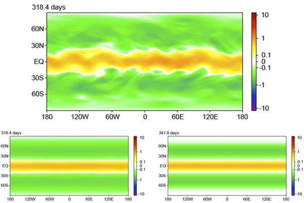
where $q=\omega +f(\varphi )$ is the absolute vorticity (the vorticity as seen in an inertial frame) and $f(\varphi )=2\mathrm{\Omega }\text{sin}\varphi$ is the Coriolis parameter familiar from the physics of Foucault’s pendulum ( $\varphi$ is the latitude and $\mathrm{\Omega }$ is the angular rotation rate of the planet). As shown in the top part of Fig. 3, a direct numerical simulation (DNS) reveals a robust equatorial jet, and its (potentially more useful) time-average mean velocity (bottom left) is captured by the CE2 model (bottom right) [29]. (See Ref. [31] for a demonstration of how CE2 can reproduce the pattern of winds in a more realistic two-layer model of the atmospheric general circulation.)

Credit: J. B. Marston

Credit: J. B. Marston

×

Stratification into quasi-2D flows, and shearing by the jets, act together to weaken the nonlinearities in large-scale flows, pulling apart vorticity before it can accumulate into highly nonlinear eddies. It is these features of the general circulation that distinguish it from the highly nonlinear problem of 3D isotropic and homogenous turbulence [32].

Additional insights can be gained from the spectrum of kinetic energy fluctuations. In both simulations of the general circulation with and without the eddy-eddy interaction [33], and in the real atmosphere [34,35], there is a $r^3$ power-law decay for length scales $r$ less than the eddy length scale (of order $1000\text{km}$). Commonly, this power-law decay is explained by invoking a cascade of enstrophy towards small scales [8,36]; however, no such cascade can occur in the absence of eddy-eddy interactions. Furthermore, in the real atmosphere there is no inertial range for which eddy-eddy interactions dominate [37]. Rather, other contributions to the spectrum stemming from the conversion of potential to kinetic energy, and friction, are important [38,39]. Thus macroturbulence can organize by mechanisms other than the enstrophy cascade. For this reason, cascades are likely more important for oceans currents than for the atmosphere.

Direct statistical approaches to large-scale atmospheric and oceanic currents lead to insights into the key physics governing the observed structures. It is still unclear, however, how applicable such approaches are and whether they can advance to become quantitatively accurate theories of the general circulation, possibly even replacing traditional techniques of direct numerical simulation. There is thus a pressing need for improved theoretical frameworks and tools to better describe nonequilibrium statistical physics. Will near-equilibrium theories prove valuable in the description of real geophysical flows? Are there general principles of nonequilibrium statistical physics waiting to be discovered? Can quantitatively accurate closures be found? Is it possible to extend direct statistical simulation to general circulation models that are complex enough to address questions such as how the storm tracks and ocean currents will shift as the climate changes?

Beyond the problems of large-scale circulation discussed here, there are many other intellectually challenging, and at the same time practically important, problems in the climate system that need deeper understanding, and concepts from statistical physics may play an important role here too. The largest uncertainty in climate models comes from limits to our understanding and modeling of clouds [40]. Clouds are vexing for models because they interfere with both incoming visible and outgoing infrared radiation, and the nature of their interaction with the radiative transfer of energy varies with cloud type (Fig. 4). Clouds are also problematic because cloud processes operate at length scales ranging from nanometer-size aerosol particles, to convection and turbulence at intermediate scales (see Ref. [41]), to clustering of clouds at scales of hundreds of kilometers. Stochastic models of clouds, where a randomly fluctuating field is introduced to model their transient nature, show promise, and realize another vision of Lorenz [42]: “I believe the ultimate climate models … will be stochastic, ie. random numbers will appear somewhere in the time derivatives.” Such models may also be amenable to direct statistical solution.

Credit: NASA Earth Observatory

Credit: NASA Earth Observatory

×

Understanding the complex dynamics of the ice sheets in Greenland and Antarctica is another pressing problem. In a climate that warms, ice that is currently resting on land will flow into the oceans, raising sea levels, but the flows are irregular and a source of continuing surprise. The ice sheets themselves are viscous fluids, but the boundary conditions at their bases and edges are especially complicated and not yet realistically captured by models [43].

On long time scales, the varied responses of the carbon cycle—the flow of carbon between reservoirs such as the air, oceans, and biosphere—to climate change become increasingly important. Ice core records show that the concentration of atmospheric carbon dioxide and methane are closely coupled to global temperatures, but the mechanisms and timescales of the couplings are unclear. Changes in vegetation will also affect the amount of light that land surfaces reflect back out into space (the fraction known as the “albedo”) as well as the transpiration of water into the air. A well-understood framework captures the mathematics of feedbacks [44], but quantitative models for many feedback processes remain primitive, with many uncertainties. Here again statistical physics may provide a useful framework for the inclusion of unresolved processes.

The many sciences of climate are increasingly important. To understand and accurately predict climate at this detailed level—if that is even possible—will require sustained interdisciplinary input from applied mathematics, astrophysics, atmospheric science, biology, chemistry, ecology, geology, oceanography, and physics, as well as guidance from the social sciences. There are many outstanding problems that would benefit from attention by physicists, and the urgency to solve these problems will likely only grow with time.

I thank Freddy Bouchet, Grisha Falkovich, Paul Kushner, Glenn Paquette, Wanming Qi, Tapio Schneider, Steve Tobias, and Peter Weichman for helpful discussions, and Lee Pedersen for tracking down the quote by Robert Heinlein. I would also like to thank the Aspen Center for Physics for its support of the 2005 Workshop on “Novel Approaches to Climate” and the Kavli Institute for Theoretical Physics for its hospitality during the 2008 program on the “Physics of Climate Change.” This work was supported in part by NSF grant Nos. DMR-065619 and PHY-0551164.

References

- Robert A. Heinlein, Time Enough for Love: The Lives of Lazarus Long (G. P. Putnam & Sons, New York, 1973)[Amazon][WorldCat]
- E. N. Lorenz, The Nature and Theory of the General Circulation of the Atmosphere, Vol. 218 (World Meteorological Organization, Geneva, 1967)
- David Archer, Global Warming: Understanding the Forecast (Wiley-Blackwell, Malden, 2006)[Amazon][WorldCat]
- Isaac M. Held, Bull. Am. Met. Soc. 86, 1609 (2005)
- James Y-K Cho and Lorenzo M Polvani, Phys. Fluids 8, 1531 (1996)
- F. P. Bretherton and D. B. Haidvogel, J. Fluid Mech. 78, 129 (1976)
- C. E. Leith, Phys. Fluids 27, 1388 (1984)
- R. H. Kraichnan and D. Montgomery, Rep. Prog. Phys. 43, 547 (1980)
- G. K. Batchelor, Phys. Fluids 12, (Suppl. 2) 233 (1969)
- J. Miller, Phys. Rev. Lett. 65, 2137 (1990)
- Jonathan Miller, Peter B. Weichman, and M. C. Cross, Phys. Rev. A 45, 2328 (1992)
- R. Robert and J. Sommeria, J. Fluid Mech. 229, 291 (1991)
- A Naso, P. H. Chavanis, and B Dubrulle, Eur. Phys. J. B 77, 187 (2010)
- Peter B. Weichman and Dean M. Petrich, Phys. Rev. Lett. 86, 1761 (2001)
- Peter B. Weichman, Phys. Rev. E 73, 036313 (2006)
- Freddy Bouchet and Eric Simonnet, Phys. Rev. Lett. 102, 094504 (2009)
- Antoine Venaille and Freddy Bouchet, Phys. Rev. Lett. 102, 104501 (2009)
- Freddy Bouchet and Antoine Venaille (unpublished)
- Garth W. Paltridge, Quart. J. Roy. Meteor. Soc. 101, 475 (1975)
- Garth W. Paltridge, Nature 279, 630 (1979)
- Garth W. Paltridge, Quart. J. Roy. Meteor. Soc. 127, 305 (2001)
- Roderick Dewar, J. Phys. A 36, 631 (2003)
- R. C. Dewar, J. Phys. A 38, 371 (2005)
- E. T. Jaynes, Phys. Rev. 106, 620 (1957)
- E. T. Jaynes, Phys. Rev. 108, 171 (1957)
- G. Grinstein and R. Linsker, J. Phys. A 40, 9717 (2007)
- S. Bruers, J. Phys. A 40, 7441 (2007)
- Glenn C. Paquette, arXiv:1011.3788
- S. M Tobias, K Dagon, and J. B Marston, Astrophys. J. 727, 127 (2011)
- Uriel Frisch, Turbulence: The Legacy of A. N. Kolmogorov (Cambridge University Press, Cambridge, 1995)[Amazon][WorldCat]
- J. B. Marston, Chaos 20, 041107 (2010)
- Tapio Schneider and Christopher C. Walker, J. Atmos. Sci. 63, 1569 (2006)
- P. A. O’Gorman and T. Schneider, Geophys. Res. Lett. 34, 22801 (2007)
- G. J. Boer and T. G. Shepherd, J. Atmos. Sci. 40, 164 (1983)
- G. D. Nastrom and K. S. Gage, J. Atmos. Sci 42, 950 (1985)
- Rick Salmon, Lectures on Geophysical Fluid Dynamics (Oxford University Press, New York, 1998)[Amazon][WorldCat]
- S. J. Lambert, Monthly Weather Review 115, 1295 (1987)
- D. M. Straus and P. Ditlevsen, Tellus A 51, 749 (1999)
- G. K. Vallis, in Non-linear Phenomena in Atmospheric and Oceanic Sciences, edited by G. F. Carnevale and R. T. Pierrehumbert (Springer, Berlin, 1992)[Amazon][WorldCat]
- G. L. Stephens, J. Climate 18, 237 (2005)
- G. Ahlers, Physics 2, 74 (2009)
- E. N. Lorenz, in The Physical Basis of Climate and Climate Modeling, WMO GARP Publication Series. No. 16 (World Meteorological Organization, Geneva, 1975)
- D. G. Vaughan and R. Arthern, Science 315, 1503 (2007)
- Gerard Roe, Annu. Rev. Earth Planet. Sci. 37, 93 (2009)